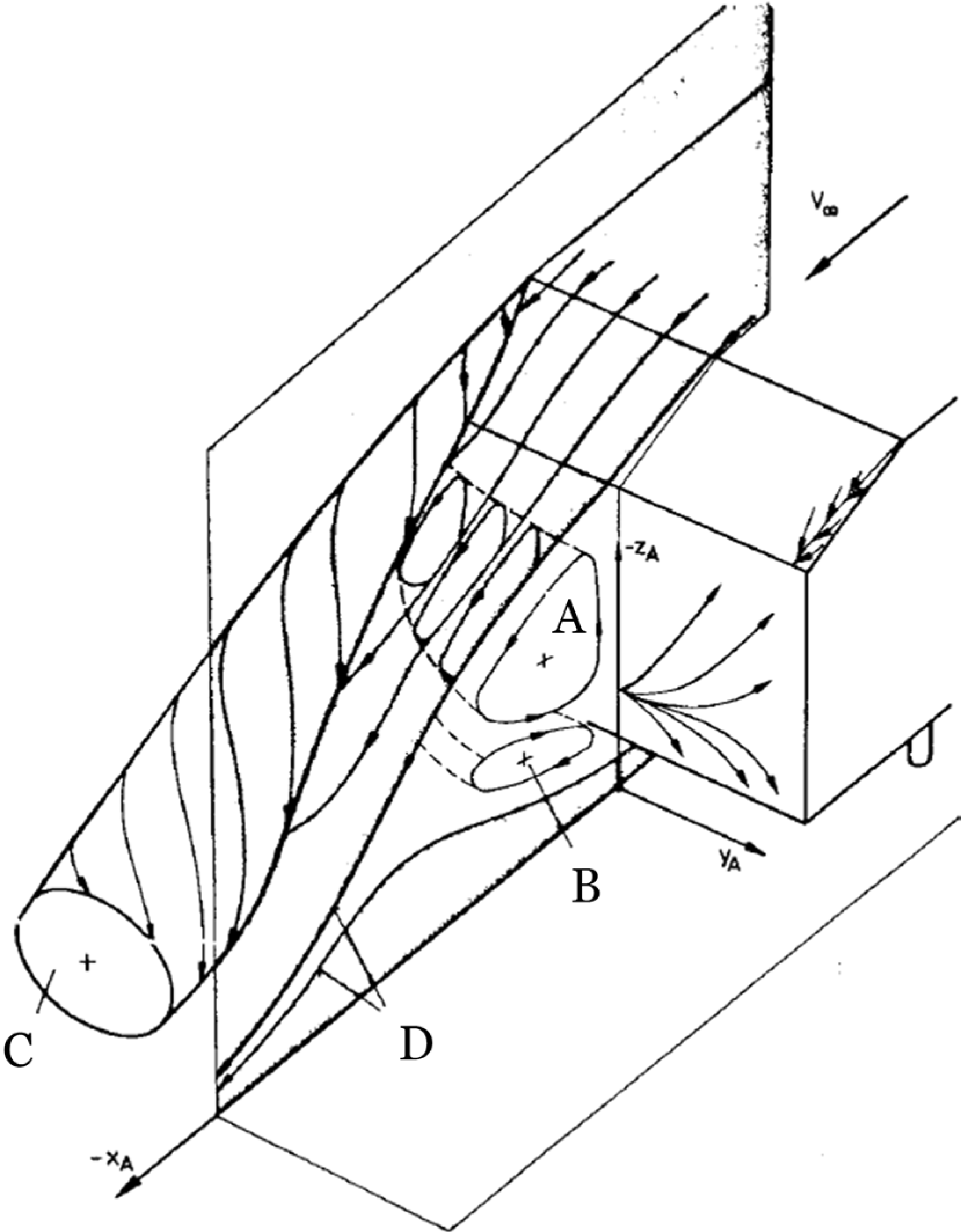
Vortices behind a car-like object. From Ahmed, Ramm & Faitin: "Some salient features of the time-averaged ground vehicle wake" (1984). Tech. rep., Society of Automotive
Engineers Inc, Warrendale, PA.

A different take on viscosity

Preamble: This article focuses on the most common conditions for steady-state air and water flow. A flow expert will be perfectly right in saying: "Yes, but...". Readability has been assigned top priority.

Also note that the material property "fluid viscosity" can be described by two values: the "dynamic viscosity" (common symbol: μ) and the "kinematic viscosity" (common symbol: ν). The latter is simply the former divided by the density.

Imagine a xylophone block which emits sound at the bending frequency of the block. For that to happen, the block material must have a certain stiffness. You may express that stiffness as its reciprocal value, which would be its flexibility. Then imagine this flexibility moving towards zero. The bending frequency will increase until you cannot hear anything. When the flexibility reaches zero, the block has no bending frequency at all. You cannot hear that, either. Zero or near-zero does not make much of a difference.

The same thing with the internal damping of the block material. When the internal damping is sufficiently low, other kinds of damping take over. Still not much of a difference between zero and near-zero.

You would expect all material property values to behave like that. Fluid viscosity - the ratio between shear force and shear velocity - is different. Already in 1752, Jean le Rond d'Alembert identified this paradox: When moving an object through air at standstill, the drag is much higher than expected from the known level of air viscosity.

The resolution of d'Alembert's paradox is to recognize that the equations governing fluid behavior (the Navier-Stokes equations) are extremely nasty. I'll write them here for the case of incompressibility, a single phase and no thermal effects (and I'll use Einstein notation in order not to blur the basics):

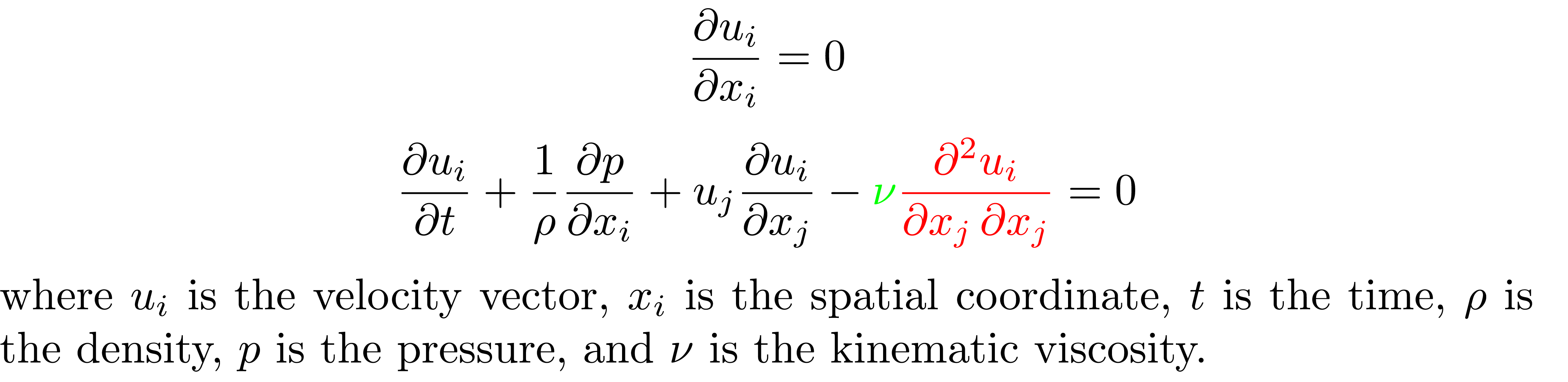
The kinematic viscosity ν (shown in green) engages or disengages the red term. If ν is zero, you only have the black terms. The black subset constitutes the equations for a so-called potential flow. Contrary to the full set of equations, the black subset is not nasty at all. But potential flow will not predict any drag (shear velocities generate no shear forces).

Potential flow is the nicest flow that never was. If you can turn the blind eye to any drag effect, you can draw wonderful conclusions from the simple theory of potential flow. However, potential flow will always slide freely along any wall. Real liquids never do. Real liquids have zero velocity at any wall.

There will always be a competition between the flow characteristics near a wall and the flow away from walls. Sufficiently close to a wall, the red term of the Navier-Stokes equations above will come into action for any nonzero value of ν. When the fluid viscosity gets smaller and smaller, the so-called boundary layer gets thinner and thinner. However, the effects of the boundary layer also get more and more dramatic (explaining d'Alembert's paradox).

The established term for this drama is "turbulence". Viscous (that is, non-potential) flow without turbulence is called laminar flow. Referring to the preamble above, I'll be simplistic: Turbulent flow is the rule, laminar flow is the exception. A flow will only be laminar for small velocities, small dimensions or a large ν.

This basic vocabulary allows for the introduction of an old split in the history of fluid mechanics:

• Tubes, pipes and the like have walls all over, especially where the fluid came from. Therefore, all regions are affected by turbulence. This is called internal flow.
• Objects moving through a fluid (cars, airplanes, etc.) create a flow in which some regions are unaffected by walls. You will have turbulence near the object and potential flow away from it. This is called external flow.

The full Navier-Stokes equations have the strange property that extremely time-dependent solutions emerge from time-independent problems. You could say that turbulence and nastiness is the same thing.

How can one cope with that? One can

1. Solve the equations anyway. Only the biggest and most modern supercomputers can do this. The essential result surprises at least me: The turbulence that you observe in real life exists in the computer, too. Many other material properties cause trouble because they are only linear in a narrow range. Also in this context, ν is something special: However ugly its effects, ν is in itself extremely linear.
2. Give up computing and rely on experimental observations. One will then see that
   Big whirls have little whirls
   that feed on their velocity;
   And little whirls have lesser whirls,
   and so on to viscosity. ― Lewis Fry Richardson
   A "whirl" is the same thing as a "vortex". They look like hurricanes on a weather map. Behind a moving object in air, you will typically see vortices as big as the object itself (as shown on the illustration up left). Vortices contain rotational kinetic energy. They are, however, unstable and will decompose into increasingly smaller vortices. When the vortices are small enough, their external boundaries will rub so much against each other that the kinetic energy dissipates into heat.
3. Solve some other equations instead. If you time-average the Navier-Stokes equations, ν is replaced by a "turbulent ν" depending nonlinearly on the solution fields themselves. If you introduce the turbulent kinetic energy k and the turbulent dissipation ε as new solution fields (additional to average velocity and average pressure), you have removed the nastiness of the Navier-Stokes equations (partly due to "turbulent ν" being sufficiently larger than ν itself). You will now get a steady-state solution from a steady-state problem.

Approach number 3 is called RANS: Reynolds-Averaged Navier-Stokes. You cannot do RANS without entering constants and/or procedure modifications that originate from fitting calculated solutions to experimental data. Even with RANS, turbulence simulations are dirty business. But with offerings like SimScale, RANS-based simulations are within anyone's reach.

Chances are, you have already loaded a template in SimScale and done a RANS-based simulation. This article intends to help you understand what you did before you knew that you had a choice.

A subsequent article will tell you about the choices that you actually have.